Transformer详细解读和代码实现

2022年12月10日

文章目录

1. 嵌入层 Embedding
2. 位置编码 Positional Encoding
3. 带缩放的点积注意力机制 Scaled Dot-Product Attention
4. 自我注意力和padding掩码 Self-Attention and Padding Mask
5. 解码器输入的后续掩码 Subsequent Mask for Decoder Input
6. 多头注意力 Multi-Head Attention
7. 分位置的前馈机制 Position-wise Feed-Forward
8. 编码器 encoder
9. EncoderBlock
10. 解码器 Decoder
11. DecoderBlock
12. Transformer
13. 应用场景 Translator
14. 参考文献

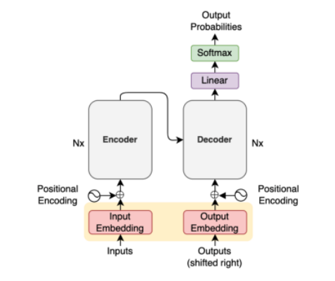
在本文中,我想讨论一下基于 Transformer 神经网络的代码细节，
因为很多人看了Transformer的理论架构以后还是云里雾里的，
所以你必须了解代码细节才能更深入的掌握Transformer架构。
这个架构是在这篇文章中提出《Attention Is All You Need》，由Ashish Vaswani等人撰写。
Transformer已经有代码实现，我已经在参考部分列出了其中一些。在阅读这些源代码时,我学习了一些技巧,这些技巧并未写在论文中，
所以我们想专门写一篇教程来介绍代码细节。

在下文中,我使用PyTorch编写每个组件的细节。
最后,我将所有模块组装起来，构成完整的Transformer。

嵌入层 Embedding

嵌入层的目的是将词索引转换为可计算的向量，比如“你”这个词，在词典中索引是5，
代表第五个词，经过嵌入层后， 5转换为一个向量，比如 $X = (0.1, 0.2, 0.11, -0.2, ..., 0.33)$

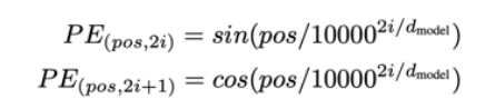
位置编码 Positional Encoding

位置编码就是将词的位置信息转换为可计算的向量，
用 pos 代表词位置， i 代表维度，
我们可以使用如下公式计算位置编码：

我们可以用下面的代码来理解位置编码：

import math
import torch

pe = torch.zeros(max_positions, dim_embed)

for pos in range(max_positions):
    for i in range(0, dim_embed, 2):
        theta = pos / (10000 ** (i / dim_embed))
        pe[pos, i    ] = math.sin(theta)
        pe[pos, i + 1] = math.cos(theta)

然而使用循环是非常耗时的，所以我们利用矩阵的并行计算原理，
可以重写上面的代码：


import math
import torch
import torch.nn as nn
from torch import Tensor

class PositionalEncoding(nn.Module):
    def __init__(self, max_positions: int, dim_embed: int, drop_prob: float) -> None:
        super().__init__()

        assert dim_embed % 2 == 0

        # Inspired by https://pytorch.org/tutorials/beginner/transformer_tutorial.html
        position = torch.arange(max_positions).unsqueeze(1)
        dim_pair = torch.arange(0, dim_embed, 2)
        div_term = torch.exp(dim_pair * (-math.log(10000.0) / dim_embed))

        pe = torch.zeros(max_positions, dim_embed)
        pe[:, 0::2] = torch.sin(position * div_term)
        pe[:, 1::2] = torch.cos(position * div_term)
        
        # 添加batch维度
        pe = pe.unsqueeze(0)
        
        # 整个学习阶段， 位置信息是不变的， 注册为不可学习的数据
        self.register_buffer('pe', pe)
        
        self.dropout = nn.Dropout(p=drop_prob)
        
    def forward(self, x: Tensor) -> Tensor:
        # 计算每个batch的最大句子长度
        max_sequence_length = x.size(1)
        
        # 词向量中添加位置信息
        x = x + self.pe[:, :max_sequence_length]
        x = self.dropout(x)
        return x

这一行代码看起来有些复杂： div_term = torch.exp(dim_pair * (-math.log(10000.0) / dim_embed)) ,
我们用数学公式写出来就不复杂了：

带缩放的点积注意力机制 Scaled Dot-Product Attention

带缩放的点积注意力机制顾名思义就是利用两个词向量的点乘来反映两者的相关性，缩放（Scaled）意味着我们将点乘结果除以词向量维数的平方根。

这里的attention机制，相比于经典的Dot-product Attention其实就是多了一个scale项。这里的作用是啥呢？当d比较小的时候，要不要scale都无所谓，但是当d比较大时，内积的值的范围就会变得很大，不同的内积的差距也会拉大，这样的话，再经过softmax进一步的扩大差距，就会使得得到的attention分布很接近one-hot，这样会导致梯度下降困难，模型难以训练。在Transformer中，d=512，算比较大了，因此需要进行scaling。

import torch
import torch.nn as nn
import torch.nn.functional as F
from torch import Tensor

def attention(query: Tensor, key: Tensor, value: Tensor, mask: Tensor=None) -> Tensor:
    sqrt_dim_head = query.shape[-1]**0.5

    scores = torch.matmul(query, key.transpose(-2, -1))
    scores = scores / sqrt_dim_head
    
    if mask is not None:
        scores = scores.masked_fill(mask==0, -1e9)
    
    weight = F.softmax(scores, dim=-1)    
    return torch.matmul(weight, value)

自我注意力和padding掩码 Self-Attention and Padding Mask

注意力机制就是产生一个权重矩阵，如下图所示，红色部分就是权重比较大的部分。

但是由于我们使用了Padding，就是较短的句子会被空白符替代，空白符不应该参与到权重计算中，所以我们在mask中，对于空白位置使用很大的负数，
这样经过softmask后，权重趋近于0，看起来权重矩阵就如下图：

解码器输入的后续掩码 Subsequent Mask for Decoder Input

解码器的输入中，我们使用mask来隐藏后续位置的信息。我们看下下面这个序列：

1	[<SOS>, 'Bonjour', 'le', 'monde', '!']

对于'Bonjour'，不应该使用之后的信息 'le', 'monde', '!', 所以它的注意力掩码就是[1, 1, 0, 0, 0]。
也就是说，在计算第一个位置的注意力值时,我们忽略第二个位置和之后的位置。在计算第二个位置的值时,我们忽略第三个位置和其余位置，以此类推：

所以，解码器中的注意力机制是padding掩码和后续掩码的结合，在生成的注意力矩阵中，上三角是被掩盖的。

def create_masks(src_batch: Tensor, tgt_batch: Tensor) -> Tuple[Tensor, Tensor]:
    # ----------------------------------------------------------------------
    # [1] padding mask
    # ----------------------------------------------------------------------
    
    # (batch_size, 1, max_tgt_seq_len)
    src_pad_mask = (src_batch != PAD_IDX).unsqueeze(1)
    
    # (batch_size, 1, max_src_seq_len)
    tgt_pad_mask = (tgt_batch != PAD_IDX).unsqueeze(1)

    # ----------------------------------------------------------------------
    # [2] subsequent mask for decoder inputs
    # ----------------------------------------------------------------------
    max_tgt_sequence_length = tgt_batch.shape[1]
    tgt_attention_square = (max_tgt_sequence_length, max_tgt_sequence_length)

    # full attention
    full_mask = torch.full(tgt_attention_square, 1)
    
    # subsequent sequence should be invisible to each token position
    subsequent_mask = torch.tril(full_mask)
    
    # add a batch dim (1, max_tgt_seq_len, max_tgt_seq_len)
    subsequent_mask = subsequent_mask.unsqueeze(0)

    return src_pad_mask, tgt_pad_mask & subsequent_mask

多头注意力 Multi-Head Attention

下图是原论文中用到的多头注意力机制图：

在编码器中，多头注意力充当自我注意力机制( self-attention mechanism)，解码器中充当自我注意力和目标源注意力(target-source attention), 可以看下图的区别：

multiHeadAtt

上图中，在解码器中的“masked multi-head attention”，多了一个mask，因为解码器使用了mask来掩盖后续词的信息。
所以对于解码器， mask 是 padding mask 和 subsequent masks 的结合。

multi-head attention 有三个输入，分别是V、K和Q，在编码器中，这三个都是词嵌入向量，但在解码器中， V和K是编码器的输出结果，
Q是解码器的词嵌入向量。

从概念上讲,我们独立执行多个scaled dot-product attention计算, 每个头一个。
为此, 我们对 V, K, Q 执行8次独立的线性操作，但是在实际情况中，我们对这三个分别执行线性操作，
但之后将他们reshape成8个头，正如下面代码所示：

# continuation of attention.py

class MultiHeadAttention(nn.Module):
    def __init__(self, num_heads: int, dim_embed: int, drop_prob: float) -> None:
        super().__init__()
        assert dim_embed % num_heads == 0

        self.num_heads = num_heads
        self.dim_embed = dim_embed
        self.dim_head = dim_embed // num_heads

        self.query  = nn.Linear(dim_embed, dim_embed)
        self.key    = nn.Linear(dim_embed, dim_embed)
        self.value  = nn.Linear(dim_embed, dim_embed)
        self.output = nn.Linear(dim_embed, dim_embed)
        self.dropout = nn.Dropout(drop_prob)

    def forward(self, x: Tensor, y: Tensor, mask: Tensor=None) -> Tensor:
        query = self.query(x)
        key   = self.key  (y)
        value = self.value(y)

        batch_size = x.size(0)
        query = query.view(batch_size, -1, self.num_heads, self.dim_head)
        key   = key  .view(batch_size, -1, self.num_heads, self.dim_head)
        value = value.view(batch_size, -1, self.num_heads, self.dim_head)

        # Into the number of heads (batch_size, num_heads, -1, dim_head)
        query = query.transpose(1, 2)
        key   = key  .transpose(1, 2)
        value = value.transpose(1, 2)
        
        if mask is not None:
            mask = mask.unsqueeze(1)

        attn = attention(query, key, value, mask)
        attn = attn.transpose(1, 2).contiguous().view(batch_size, -1, self.dim_embed)
        
        out = self.dropout(self.output(attn))

        return out

Q, K, V 的形状从(batch_size, max_sequence_length, dim_embed)变为(batch_size, num_heads, max_sequence_length, dim_head)，
而dim_head = dim_embed // num_head。例如dim_embed = 512 且 num_heads = 8, 那么dim_head = 64。

然后，我们将attention的结果reshape成(batch_size, max_sequence_length, dim_embed)。所以，经过了多头注意力机制，
输入输出的张量形状是相同的。

mask.unsqueeze(1)的目的是给mask增加一个维度，这样不同的头使用相同的mask，在attention这个函数中， masked_fill可以实现这个目的。
最后，使用dropout.

分位置的前馈机制 Position-wise Feed-Forward

Position-wise-Feed-Forward

Position-wise Feed-Forward 给词向量增加了非线性。词向量的形状是(batch_size, max_sequence_length, dim_embed),
很多神经网络处理词向量的时候会进行flatten然后再进入前馈神经网络，我们并没有将词向量进行flatten，我们的线性操作是对每个位置进行独立的操作，
因此，这里被称为 Position-wise 。

import torch.nn as nn
from torch import Tensor

class PositionwiseFeedForward(nn.Module):
    def __init__(self, dim_embed: int, dim_pffn: int, drop_prob: float) -> None:
        super().__init__()
        self.pffn = nn.Sequential(
            nn.Linear(dim_embed, dim_pffn),
            nn.ReLU(inplace=True),
            nn.Dropout(drop_prob),
            nn.Linear(dim_pffn, dim_embed),
            nn.Dropout(drop_prob),
        )

    def forward(self, x: Tensor) -> Tensor:
        return self.pffn(x)

第一次线性操作扩大了维度。我了解这样做意味着ReLU不会丢失太多信息。
第二个线性操作将恢复原始维度。因此,我们可以继续使用相同的维度来执行其余过程。
例如在base Transformer模型中，词嵌入向量从512扩展到2048，然后再恢复到512 。

编码器 encoder

encoder

Transformer使用了多个encoder模块，从图中可以看到。

下面的代码实现了多个encoder的堆叠，但是没有实现EncoderBlock，之后才会实现。

import torch.nn as nn
from torch import Tensor
from .attention import MultiHeadAttention
from .feed_forward import PositionwiseFeedForward

class Encoder(nn.Module):
    def __init__(self,
                 num_blocks: int,
                 num_heads:  int,
                 dim_embed:  int,
                 dim_pffn:   int,
                 drop_prob:  float) -> None:
        super().__init__()

        self.blocks = nn.ModuleList(
            [EncoderBlock(num_heads, dim_embed, dim_pffn, drop_prob)
             for _ in range(num_blocks)]
        )
        self.layer_norm = nn.LayerNorm(dim_embed)
        
    def forward(self, x: Tensor, x_mask: Tensor):
        for block in self.blocks:
            x = block(x, x_mask)
        x = self.layer_norm(x)
        return x

EncoderBlock

接下来我们实现图中所示的结构。

# continuation of encoder.py

class EncoderBlock(nn.Module):
    def __init__(self,
                 num_heads: int,
                 dim_embed: int,
                 dim_pwff:  int,
                 drop_prob: float) -> None:
        super().__init__()

        # Self-attention
        self.self_atten = MultiHeadAttention(num_heads, dim_embed, drop_prob)
        self.layer_norm1 = nn.LayerNorm(dim_embed)

        # Point-wise feed-forward
        self.feed_forward = PositionwiseFeedForward(dim_embed, dim_pwff, drop_prob)
        self.layer_norm2 = nn.LayerNorm(dim_embed)

    def forward(self, x: Tensor, x_mask: Tensor) -> Tensor:
        // 图中Add节点
        x = x + self.sub_layer1(x, x_mask)
        x = x + self.sub_layer2(x)
        return x

    def sub_layer1(self, x: Tensor, x_mask: Tensor) -> Tensor:
        // 先进行norm
        x = self.layer_norm1(x)
        x = self.self_atten(x, x, x_mask)
        return x
    
    def sub_layer2(self, x: Tensor) -> Tensor:
        x = self.layer_norm2(x)
        x = self.feed_forward(x)
        return x

实际上代码和上面的概念图有区别，因为有研究认为，在进入sub layer之前先进行 normalization 更好。

所以我们采用下面的概念图：

EncoderBlock2

解码器 Decoder

我们先来实现总体流程：

decoder

import torch.nn as nn
from torch import Tensor
from .attention import MultiHeadAttention
from .feed_forward import PositionwiseFeedForward


class Decoder(nn.Module):
    def __init__(self,
                 num_blocks: int,
                 num_heads:  int,
                 dim_embed:  int,
                 dim_pffn:   int,
                 drop_prob:  float) -> None:
        super().__init__()
        // DecoderBlock 还没有实现  下面会写
        self.blocks = nn.ModuleList(
            [DecoderBlock(num_heads, dim_embed, dim_pffn, drop_prob)
             for _ in range(num_blocks)]
        )
        self.layer_norm = nn.LayerNorm(dim_embed)

    def forward(self, x: Tensor, x_mask: Tensor, y: Tensor, y_mask: Tensor) -> Tensor:
        for block in self.blocks:
            y = block(y, y_mask, x, x_mask)
        y = self.layer_norm(y)
        return y

DecoderBlock

这里是DecoderBlock的具体细节：

DecoderBlock

DecoderBlock有4个注意点：

自我注意力使用 Masked multi-head attention
目标源注意力使用 multi-head attention
使用Position-wise feed-forward 给网络加入非线性
层之间使用 residual connection 和 layer normalization ：x + Sublayer(LayerNorm(x))

class DecoderBlock(nn.Module):
    def __init__(self,
                 num_heads: int,
                 dim_embed: int,
                 dim_pwff:  int,
                 drop_prob: float) -> None:
        super().__init__()

        # Self-attention
        self.self_attn = MultiHeadAttention(num_heads, dim_embed, drop_prob)
        self.layer_norm1 = nn.LayerNorm(dim_embed)

        # Target-source
        self.tgt_src_attn = MultiHeadAttention(num_heads, dim_embed, drop_prob)
        self.layer_norm2 = nn.LayerNorm(dim_embed)

        # Position-wise
        self.feed_forward = PositionwiseFeedForward(dim_embed, dim_pwff, drop_prob)
        self.layer_norm3 = nn.LayerNorm(dim_embed)

    def forward(self, y, y_mask, x, x_mask) -> Tensor:
        // 实现residual connection
        y = y + self.sub_layer1(y, y_mask)
        y = y + self.sub_layer2(y, x, x_mask)
        y = y + self.sub_layer3(y)
        return y

    def sub_layer1(self, y: Tensor, y_mask: Tensor) -> Tensor:
        y = self.layer_norm1(y)
        y = self.self_attn(y, y, y_mask)
        return y

    def sub_layer2(self, y: Tensor, x: Tensor, x_mask: Tensor) -> Tensor:
        y = self.layer_norm2(y)
        y = self.tgt_src_attn(y, x, x_mask)
        return y

    def sub_layer3(self, y: Tensor) -> Tensor:
        y = self.layer_norm3(y)
        y = self.feed_forward(y)
        return y

Transformer

transformer

下面就是将所有模块整合成一个模块的时候了，所以下面的代码用到了以上所有的代码：

import torch.nn as nn
from torch import Tensor
from ..modules import Embedding, PositionalEncoding, Encoder, Decoder

class Transformer(nn.Module):
    def __init__(self,
                 input_vocab_size:  int,
                 output_vocab_size: int,
                 max_positions:     int,
                 num_blocks:        int,
                 num_heads:         int,
                 dim_embed:         int,
                 dim_pffn:          int,
                 drop_prob:         float) -> None:
        super().__init__()

        # Input embeddings, positional encoding, and encoder
        self.input_embedding = Embedding(input_vocab_size, dim_embed)
        self.input_pos_encoding = PositionalEncoding(
                                      max_positions, dim_embed, drop_prob)
        self.encoder = Encoder(num_blocks, num_heads, dim_embed, dim_pffn, drop_prob)

        # Output embeddings, positional encoding, decoder, and projection 
        # to vocab size dimension
        self.output_embedding = Embedding(output_vocab_size, dim_embed)
        self.output_pos_encoding = PositionalEncoding(
                                       max_positions, dim_embed, drop_prob)
        self.decoder = Decoder(num_blocks, num_heads, dim_embed, dim_pffn, drop_prob)
        self.projection = nn.Linear(dim_embed, output_vocab_size)

        # Initialize parameters
        for param in self.parameters():
            if param.dim() > 1:
                nn.init.xavier_uniform_(param)

    def forward(self, x: Tensor, y: Tensor,
                      x_mask: Tensor=None, y_mask: Tensor=None) -> Tensor:
        x = self.encode(x, x_mask)
        y = self.decode(x, y, x_mask, y_mask)
        return y

    def encode(self, x: Tensor, x_mask: Tensor=None) -> Tensor:
        x = self.input_embedding(x)
        x = self.input_pos_encoding(x)
        x = self.encoder(x, x_mask)
        return x

    def decode(self, x: Tensor, y: Tensor,
                     x_mask: Tensor=None, y_mask: Tensor=None) -> Tensor:
        y = self.output_embedding(y)
        y = self.output_pos_encoding(y)
        y = self.decoder(x, x_mask, y, y_mask)
        return self.projection(y)

最后一层使用 nn.Linear 将词向量的维数转换为output_vocab_size，这样就可以使用softmax输出词的概率。

应用场景 Translator

我们列举一个使用场景，以便你对Transformer有更深的理解，下面是一个翻译器的架构：

translater

关键的流程如下：

编码器从句子中提取特征
解码器的第一个输入是SOS(the start-of-sentence token)
解码器输出第一个词的概率
最大概率的词的词向量作为解码器的第二个输入
重复上面两个步骤
当输出EOS (end-of-sentence)时，停止

参考文献

注意
深度学习和统计咨询请加QQ 2726725926, 微信 shujufenxidaizuo
请记住我的网址: mlln.cn 或者 jupyter.cn

#深度学习

Transformer详细解读和代码实现

嵌入层 Embedding

位置编码 Positional Encoding

带缩放的点积注意力机制 Scaled Dot-Product Attention

自我注意力和padding掩码 Self-Attention and Padding Mask

解码器输入的后续掩码 Subsequent Mask for Decoder Input

多头注意力 Multi-Head Attention

分位置的前馈机制 Position-wise Feed-Forward

编码器 encoder

EncoderBlock

解码器 Decoder

DecoderBlock

Transformer

应用场景 Translator

参考文献

赞助

赞助推荐

常用工具

深度学习

友商赞助